Simulating Operational Amplifier Saturation

When imitating a real world circuit in the digital world, it is important to consider the quirks and constraints present in hardware components. This article is looking at how a software application can mimic the effects on a signal of an operational amplifier when it reaches saturation.

The incredibly versatile Operational Amplifier (Op-Amp) has many flaws and caveats that have to be considered in circuit design. When software aims to mimic a hardware design, these imperfections should be considered, and replicated as desired.

In an ideal world, Operational Amplifiers would be able to output any arbitrary voltages, but in reality they are constrained by their power supply. The peak-to-peak voltage of the outputted signal cannot go higher than the voltage of the power rails; this is called Saturation. In older op-amps, the peak-to-peak voltage of the output signal would be several volts less than the power supply’s peak-to-peak voltage, though newer op-amps can get closer to the power supply.

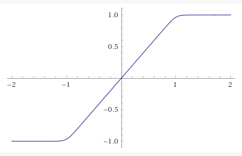
When looking at the datasheet of an Op-Amp, you’ll often see a graph that resembles something like this:

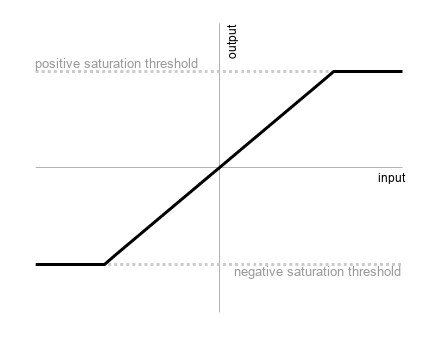The kind of Op-Amp saturation graph you see in a datasheet or in education.

This characteristic can be represented like this:

where\( \; n = \text{negative saturation voltage}\),\( \; p = \text{positive saturation voltage}\),\( \; x = \text{input signal}\),\( \; g = \text{gain}\).

In other words, the output of the op-amp is linear in regards to the input whilst between the two saturation thresholds, though once it goes above or below the positive or negative saturation levels, the output matches the saturation level.

This is an idealised version of a non-ideal op-amp, which is a strange concept. Real Op-Amp saturation doesn’t look like that, nor does an idealised Op-Amp (which wouldn’t saturate at all). This idealised version would be easy for us to simulate without doing any complicated calculation; simply clip at the saturation thresholds.

In reality, an op-amp has a slight curve as it nears saturation, and it becomes non-linear, similar to the below (which is a little exaggerated):

A slightly more realistic graph of Op-Amp saturation.

This is the characteristic that I’d like to imitate.

We can tell just by looking at it that it is a Sigmoid Function (aka any function with an ‘S’ shape.)

I’m not an expert mathematician, so I’ll often do a bit of trial and error with Wolfram Alpha to see if I can nudge an equation closer to what I’m looking for.

I eventually turned my attention to the given algebraic function:

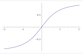The graph of \(y = \frac{x}{\sqrt{1+x^2}}\), plotted by Wolfram Alpha.

It has a fairly lacklustre performance characteristic as written; there is almost no linear region. However, I noticed that if I generalised the formula (ie to the formula below), then as n increased, the characteristic became more like the idealised op-amp saturation characteristic.

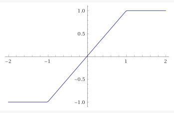The graph of \(y = \frac{x}{\sqrt[100]{1+x^{100}}}\), plotted by Wolfram Alpha.

The graph above is for \(n = 100\). When I differentiated this function, I saw that yes, the ‘linear region’ was actually linear (and not some imperceptible curve):

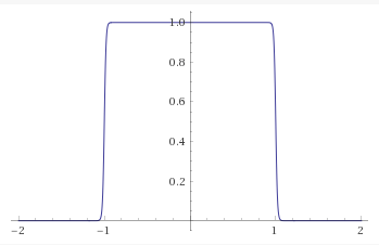First order differential of \(y = \frac{x}{\sqrt[100]{1+x^{100}}}\), plotted by Wolfram Alpha.

I played with the numbers and ended up settling with \(n = 100\). It seemed like a good medium between ‘not doing anything’ and ‘doing too much’. If I really wanted to I could measure it on an oscilloscope and try to match it exactly, but for me this was good enough.

The graph of \(y = \frac{x}{\sqrt[20]{1+x^{20}}}\), plotted by Wolfram Alpha.

To use this in your code, simply rescale your input signal so that the thresholds fall at -1 and 1, pass the rescaled signal through the function (as \(x\)), and then scale back up.

I did this for a C++ project, so my code looks like this:

float saturate(float input, float threshold) {
    float scale = input / threshold;
    return (threshold * scale) / (std::pow(1.f + std::pow(scale,20.f), 1.f/20.f));
}