A few days ago, my girlfriend Ni sent me an Excel spreadsheet that she had received, and asked me to explain to her how it was made and how it works. She’s trying to learn more about Excel to help her automate routine tasks and be more efficient with her spreadsheets.

I’m not an expert at Excel - I often just write code to do calculations for me - but I thought I’d give it a go.

The main feature that she wanted to replicate from the document was a sheet with a dropdown box allowing the user to pick a month. The sheet acted like a ‘summary’ or ‘view’ page, pulling in data from other sheets for display. It pulled from specific sheets based on the selected month.

I’ve recorded a demonstration video of the spreadsheet that Ni received. For legal reasons, I have replaced the data from that spreadsheet with junk data.

I did some searching online and managed to figure out a solution on my own, without reverse engineering the spreadsheet that Ni has sent me. Because I was curious, I reverse engineered that spreadsheet too, which I’ll write some notes about at the end of this post.

You can download a demo of what I will be creating here.

Drop Down List

The Drop Down List is a key aspect of this spreadsheet.

It’s actually remarkably simple to implement. Spreadsheet Software have a feature called ‘Data Validation’, which you can use to create a list of values that a cell can take.

In Excel

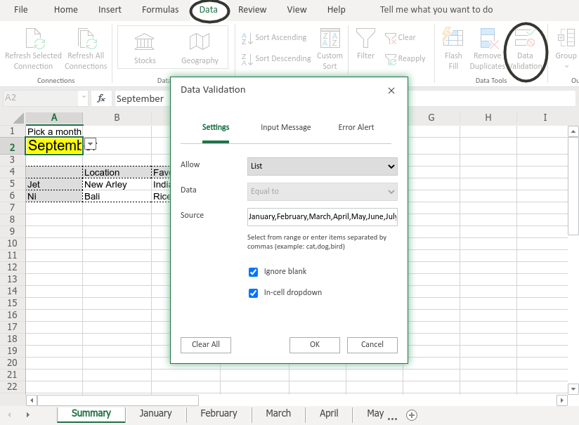Data Validation in Excel.

In Excel, you can find it by going to Data > Data Tools > Data Validation > Settings > Allow: (List), and then entering a list of allowable text, like this:

January,February,March,

If you’re inputting something that has a month and a year, Excel may try to automatically convert it from Text to a Date, which we don’t want. Either use a different text format that it won’t convert (eg 20-Jan rather than Jan-20), or explicitly set it to text (such as by typing ="Jan-20").

In LibreOffice

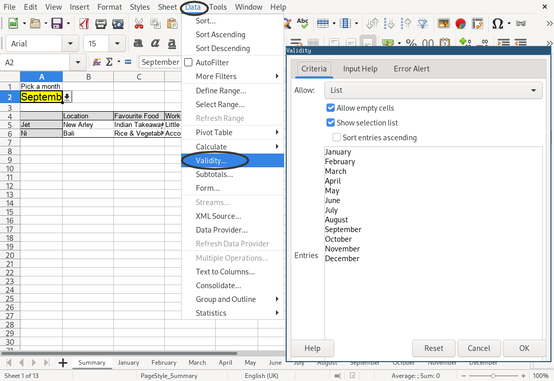Data Validation in LibreOffice.

In LibreOffice, the same feature can be found under Data > Validity > Criteria > Allow: (List). The format is much the same, but you can write the values on multiple lines rather than seperating them with semi-colons.

January
February
March

For the purposes of this guide, make sure that they match the names of the sheets that you want to pull values from.

If you’re inputting something that has a month and a year, LibreOffice may try to automatically convert it from Text to a Date, which we don’t want. Either use a different text format that it won’t convert (eg 20-Jan rather than Jan-20), or explicitly set it to text (such as by typing ="Jan-20").

The Formula

The second thing to implement this feature is a simple formula.

In my case, I have the drop down list on Cell A2, and wanted to get data from Cell B5 from each sheet.

Therefore, we want to create a formula that uses the contents of cell A2 as the name of the sheet, and references cell B5 in every sheet. We can do this using the INDIRECT() and CELL() functions, and &, the string concatenation operator.

The formula looks like this:

=INDIRECT("'" & $A$2 & "'!" & CELL("address",B5))

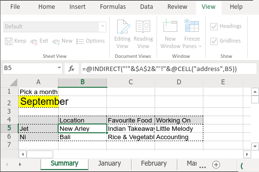The Formula in Excel.

INDIRECT() converts any entered text to a cell reference. For example, =INDIRECT("'Sheet1'!A1"), is equivalent to just having ='Sheet1'!A1.

CELL("address", <CELLREFERENCE>) converts a cell reference to a text form of it (aka it converts B5 into "B5"). I’m using this to allow us to AutoFill our formula; without it, we would write "B5" as text and it wouldn’t increment the index as we AutoFilled the formula into new cells.

The string concatenation operator (&) joins two pieces of text together. We use it to build up a cell reference (like 'January'!B5) by joining ' with the cell A2 (January), the text '!, and the address of cell B5 (B5). This cell reference comes out as text, which INDIRECT converts to a valid cell reference. Hopefully you can see us doing that in the formula!

…and you’re done!

What follows from here is just a short analysis of the spreadsheet that Ni sent me because I thought it was interesting.

The Wrong Way

When I first opened Ni’s spreadsheet, I was stumped because I couldn’t figure out how the cells were pulling in the data. When I clicked on any of the cells, there wasn’t a formula in the formula box at all. I’d never seen anything like that at all. What’s more, every sheet was ‘protected’, preventing me from editing and interfering.

Not one to be deterred, I used a Excel VBA script (that someone had shared online) to brute force the password. The script I found just unlocked the active sheet, but I modified it to return the password so that I could unlock the rest much quicker.

It turned out there were formulas in all of the cells, but that they were just hidden with formatting.

I was quite surprised and a little horrified by the formulas that I found. Initially, the whole document has seemed quite polished. It was nicely formatted, and there were even little textboxes everywhere that acted as tutorials on how to interpret the data, etc.

The actual formulas were not polished at all. They were overengineered and clunky, and it showed; when I tried to save the document, it took several seconds (on my SSD!). The document even crashed a few times as I edited the data, which I’m thinking might be something to do with the formulas (or maybe there’s something else in that document that LibreOffice didn’t like.

In short, the formula for one of the cells on the ‘summary’ sheet looks like this:

=IF($A$6="JANUARI",
    jan!A11!,
    IF($A$6="FEBRUARI",
        Feb!A11,
        IF($A$6="MARET",
            Mar!A11,
            IF($A$6="APRIL",
                Apr!A11,
                IF($A$6="MEI",
                    Mei!A11,
                    IF($A$6="JUNI",
                        Jun!A11,
                        IF($A$6="JULI",
                            Jul!A11,
                            EO12
                        )))))))

Formatting my own.

If you understand Excel Formulas enough to be able to interpret that, you’ll see that they ran out of space or something, and had to create a second hidden table all the way over at cell EO12.

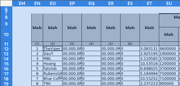Second Partial Table hidden at EO12.

The cells there contain formulas like this:

=IF($A$6="AGUSTUS",
    Agt!A11,
    IF($A$6="SEPTEMBER",
        Sep!A11,
        IF($A$6="OKTOBER",
            Okt!A11,
            IF($A$6="NOPEMBER",
                Nop!A11,
                Des!A11
            ))))

Formatting my own.

So putting that all together, they check if the contents of $A$6 is each specific month, and then reference a fixed cell on a fixed sheet.

Whilst that works, it’s quite a clumsy formula, and has flaws:

• It’s time-consuming to change for formula. For example, if they wanted to create a version of the spreadsheet for the English language (rather than Indonesian), they have to redo all of the formulas in addition to renaming the sheets and updating the data validation text-box.

• It’s hard to change the formula. For instance, if we want to change our referenced cell from A11 to B11, we have to change it in 12 places. The same problem occurs if we want to change where the month reference ($A$6) is.

• It’s easy to make a mistake in the formula. For example, it would be have been very easy to accidentally type Sep!A12 rather than Sep!A11 and not notice. The formula would work for every case except September, so might go unnoticed for a long time.

• When you have a lot of cells with long formulas like this, the spreadsheet becomes very large. It takes several seconds for me to save the document, and it crashed LibreOffice multiple times whilst I was editing data. I have never had LibreOffice crash before now.

The only advantage I can see for this kind of formula is that it is very easy to understand for a beginner.